When I initially started writing this post, I intended to focus on the most widely used Excel formulas for business. All I could think of was very basic formulas like SUM, AVG, IF, AND and so on. Of course, these are very basic, but without them you can’t really do anything else. However, you probably know those formulas well enough, and they barely scratch the surface of what you can do in Excel. As a result, in this post, I will take a look at some of the best Excel formulas that are still useful in business situations, but won’t be familiar to every single Excel user in the world.
Conditional Arithmetic
Knowing how to use a function like SUM is all well and good if you are always adding data from all the rows in your dataset. However, at some point you will want to add conditions that determine which rows you want to add together. To do this, you can use the functions such as SUMIF, COUNTIF or AVERAGEIF.
In the below example, we want to find the total revenue for all orders valued above $30,000. The formula used is: =SUMIF(F2:F24,”>30000″,F2:F24).
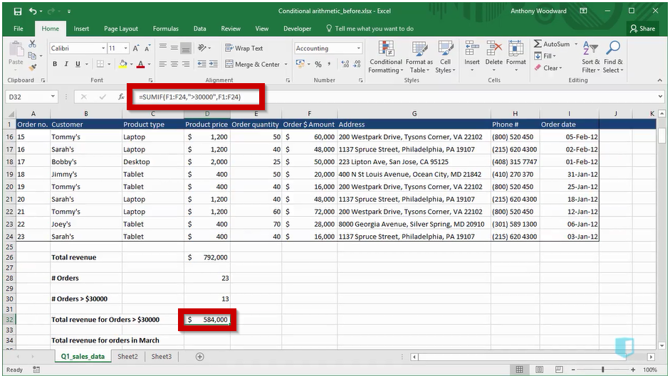
In this case, the SUMIF formula takes three arguments:
- The range we want to check, which is the order amounts in column F.
- The condition we want to check in that range, which is greater than 30,000. Notice that the condition is placed in double quotes.
- The sum range, which is the range of values we want to sum when the condition is satisfied. In this case this is also the order amount. The result, in cell D32 tells us that orders of over $30,000 brought in total revenue of $584,000.
If you want to check multiple conditions, you can do that just as easily, using the functions SUMIF, COUNTIFS, or AVERAGEIFS. Below we use COUNTIFS to count the number of orders that meet two conditions. In this case, the function used is: =COUNTIFS(C2:C24,”Tablet”,I2:I24,”>=1/3/2012″).
The first condition is that “Product Type”, in Column C is “Tablet”. The second is that “Order Date”, in Column I is on or after 1st March 2012. COUNTIFS counts the number of rows where both conditions are satisfied, which turns out to be 3.

Conditional functions such as these are very common, and are easy to apply when you understand the three main arguments you will use: the condition you are checking, the range you are checking it over, and the sum range which you sum when the condition is satisfied.
Fill Commands
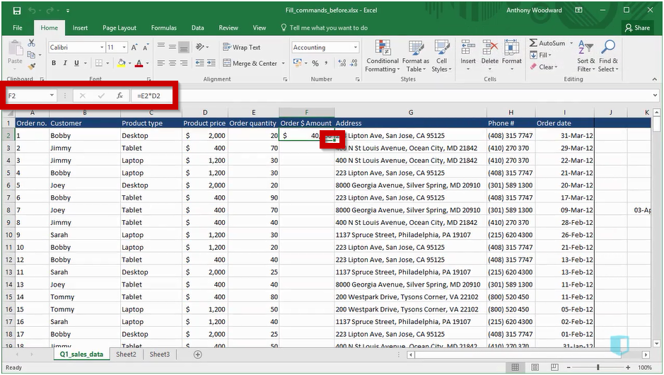
When you place a formula into a single cell, you will very often want to fill the formula along a column or a row. In the example below, we have created a formula for the order amount and want to copy it down the rest of the column. There are a few different ways of doing this.
The method you might be familiar with, or at least the one I use most often, uses the mouse. You simply double click the small square in the bottom right corner of cell F2, and the formula, as well as the cell formatting, is copied down to the last row in this data array. This is easily the best option when you are working with a large dataset, however it is not perfect. For example, double clicking only copies down, not across.
For smaller examples, or situations where you need to copy across, you can use the Fill Down and Fill Right commands. This requires you to preselect the cells you are going to fill, as seen below. As you can see, we are copying a formula across a row here.
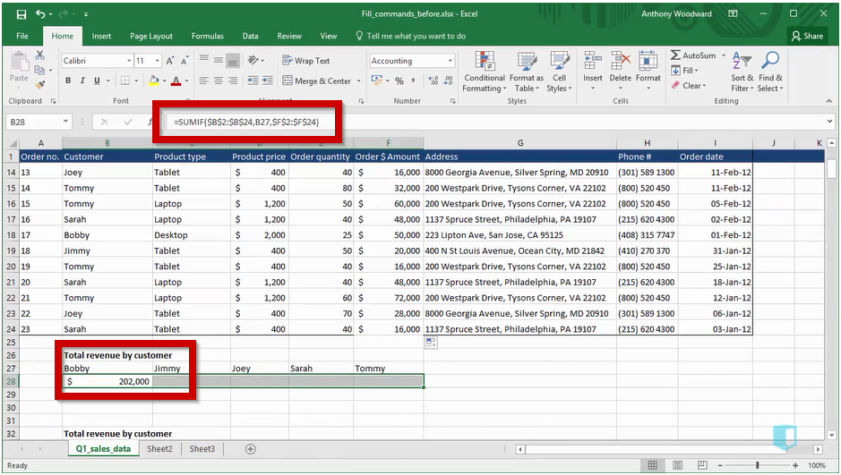
Once you have selected the cells, you can fill right using the keyboard shortcut Control + R, or fill down using Control + D. You can also use the fill options to the right of the Home tab. This method has the advantage that you can use keyboard shortcuts instead of the mouse. If you have completed the shortcuts lessons from Kubicle, the chances are you don’t use the mouse very much, so this can be useful to you.
Array Formulas
In the previous post, we looked at conditional arithmetic, such as SUMIF and COUNTIF. These formulas are inbuilt versions of array formulas. Array formulas perform multiple calculations on an array of cells. Although using inbuilt functions where possible is generally the best option, there are some situations where this will not be possible. For example, unless you have Excel 2016, there is no MAXIF or MINIF function. In that case you will need to use an array function.
Below we see an array function which finds the maximum order quantity for tablet products. The formula used is: {=MAX(IF(C2:C24=D32,E2:E24))}.
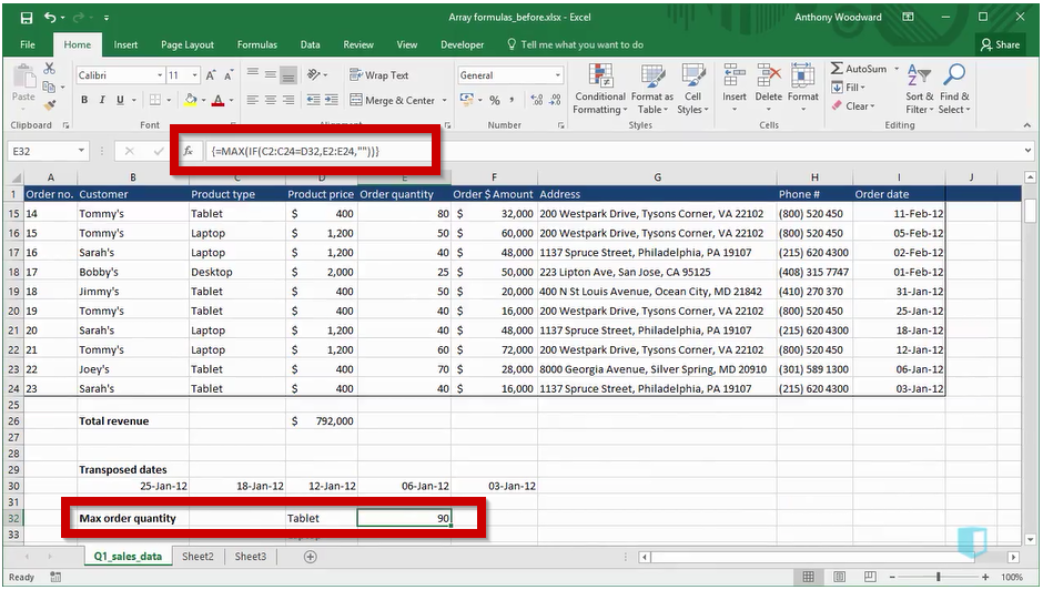
To understand how this function works, let’s look at it from the inside out. The if function checks if the product type, in column C is equal to tablet, stored in cell D32. If the product is a tablet, then the order quantity is returned. The if function therefore produces a list of order quantities for Tablets, and the max function finds the max order quantity for tablet products. It is important to remember that when using an array function, you must place curly brackets around the formula. This can be achieved by pressing Control + Shift + Enter when creating the formula instead of just Enter.
Using array functions such as this is obviously trickier than using an inbuilt function such as SUMIF, but it is necessary in a few situations where there is no inbuilt function. In general array formulas can be a tricky part of Excel, but if you can understand them, your Excel abilities will be above a lot of other Excel users.
Information Functions
Your natural analytic instinct when you get a shiny new dataset is often to go and start doing some analysis work right away. However, it’s generally best to stop briefly and make sure everything is as it should be. There are a number of information functions that you can use to find out more about your dataset. In fact there are too many to cover in a post like this, but I will look at one important one, ISBLANK.
Missing data is surely the scourge of any data analyst. Excel cannot tell you what to do about it, but it can at least help you find it, using the function ISBLANK. Like many information functions, this is often used inside an IF statement. Below is an example of this, using the formula:
=IF(ISBLANK(E3), “Re-check order quantity”, “OK”).
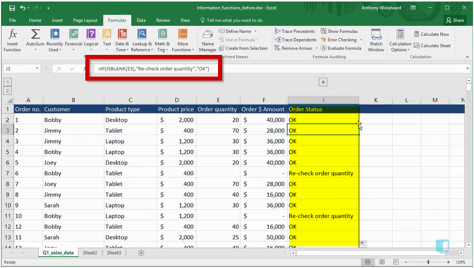
The ISBLANK formula checks if the order amount is blank, while the if statement creates an appropriate message to place in the Order Status column. This allows you to easily identify rows that do not have an order quantity, so you can do something about them.
There are many other similar functions available that work in similar ways. Common ones you might encounter are ISERROR, ISNUMBER or ISTEXT. They can all be used to check the state of your dataset before you launch into analysing your data.
Generally speaking, you should use these functions only at the start of a project. Once you begin your analysis, you should always know what type of data you have, and therefore have no need for them. Using these functions to check through your data at the start of a project can be a big time saver. The last thing you want is to build a large workbook, perhaps with some complex model, and then find your results don’t make any sense because you have some blank data you hadn’t noticed initially.
Conclusion
This concludes our look at some of the most important formulas in Excel, beyond the basics. Knowing these formulas will move you up a level on the Excel food chain, above anyone who can work with the most common, but also most basic functions in Excel. They cover a broad variety of situations, but they all can help you accomplish more advanced tasks, or save time on more common tasks. It goes without saying that these are not the only formulas of interest in Excel. In the future, we’ll look at some other useful functions for business that are less mainstream.


